6.2 KiB
Overview
The following “book” of targets “Physics-Based Deep Learning” techniques, i.e., methods that combine physical modeling and numerical simulations with deep learning (DL). Here, DL will typically refer to methods based on artificial neural networks. The general direction of Physics-Based Deep Learning represents a very active, quickly growing and exciting field of research.
Motivation
From weather forecasts (? ) over X, Y, … more … to quantum physics (? ), using numerical analysis to obtain solutions for physical models has become an integral part of science.
At the same time, machine learning technologies and deep neural networks in particular, have led to impressive achievements in a variety of field. Among others, GPT-3 has recently demonstrated that learning models can achieve astounding accuracy for processing natural language. Also: AlphaGO, closer to physics: protein folding… This is a vibrant, quickly developing field with vast possibilities.
The successes of DL approaches have given rise to concerns that this technology has the potential to replace the traditional, simulation-driven approach to science. Instead of relying on models that are carefully crafted from first principles, can data collections of sufficient size be processed to provide the correct answers instead?
Very clear advantages of data-driven approaches would lead to a “yes” here … but that’s not where we stand as of this writing. Given the current state of the art, these clear breakthroughs are outstanding, the proposed techniques are novel, sometimes difficult to apply, and significant difficulties combing physics and DL persist. Also, many fundamental theoretical questions remain unaddressed, most importantly regarding data efficienty and generalization.
Over the course of the last decades, highly specialized and accurate discretization schemes have been developed to solve fundamental model equations such as the Navier-Stokes, Maxwell’s, or Schroedinger’s equations. Seemingly trivial changes to the discretization can determine whether key phenomena are visible in the solutions or not.
{admonition} Goal of this document :class: tip Thus, a key aspect that we want to address in the following in the following is: - explain how to use DL, - and how to combine it with existing knowledge of physics and simulations, - **without throwing away** all existing numerical knowledeg and techniques!
Rather, we want to build on all the neat techniques that we have at our disposal, and use them as much as possible. I.e., our goal is to reconcile the data-centered viewpoint and the physical simuation viewpoint.
Also interesting: from a math standpoint … ‘’just’’ non-linear optimization …
Categorization
Within the area of physics-based deep learning, we can distinguish a variety of different approaches, from targeting designs, constraints, combined methods, and optimizations to applications. More specifically, all approaches either target forward simulations (predicting state or temporal evolution) or inverse problems (e.g., obtaining a parametrization for a physical system from observations).
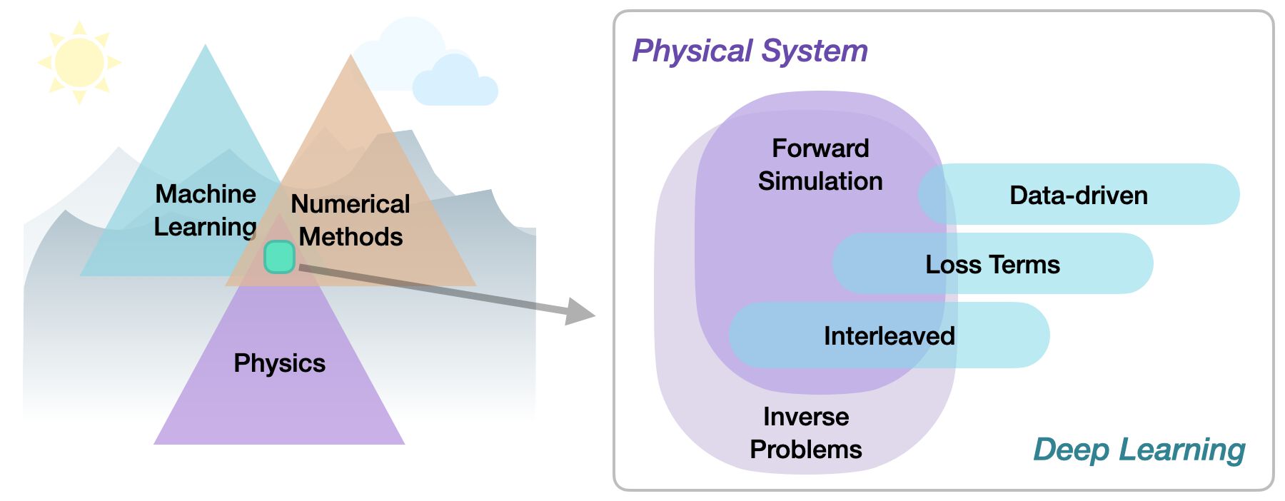
No matter whether we’re considering forward or inverse problem, the most crucial differentiation for the following topics lies in the nature of the integration between DL techniques and the domain knowledge, typically in the form of model euqations. Looking ahead, we will particularly aim for a very tight intgration of the two, that goes beyond soft-constraints in loss functions. Taking a global perspective, the following three categories can be identified to categorize physics-based deep learning (PBDL) techniques:
Data-driven: the data is produced by a physical system (real or simulated), but no further interaction exists.
Loss-terms: the physical dynamics (or parts thereof) are encoded in the loss function, typically in the form of differentiable operations. The learning process can repeatedly evaluate the loss, and usually receives gradients from a PDE-based formulation.
Interleaved: the full physical simulation is interleaved and combined with an output from a deep neural network; this requires a fully differentiable simulator and represents the tightest coupling between the physical system and the learning process. Interleaved approaches are especially important for temporal evolutions, where they can yield an estimate of future behavior of the dynamics.
Thus, methods can be roughly categorized in terms of forward versus inverse solve, and how tightly the physical model is integrated into the optimization loop that trains the deep neural network. Here, especially approaches that leverage differentiable physics allow for very tight integration of deep learning and numerical simulation methods.
The goal of this document is to introduce the different PBDL techniques, ordered in terms of growing tightness of the integration, give practical starting points with code examples, and illustrate pros and cons of the different approaches. In particular, it’s important to know in which scenarios each of the different techniques is particularly useful.
A brief history of PBDL in the context of Fluids
First:
Tompson, seminal…
Chu, descriptors, early but not used
Ling et al. isotropic turb, small FC, unused?
PINNs … and more …
Deep Learning and Neural Networks
Very brief intro, basic equations… approximate f(x)=y with NN …
Details in Deep Learning book
Notation and Abbreviations
Unify notation… TODO …
Math notation:
| Symbol | Meaning |
|---|---|
| x | NN input |
| y | NN output |
| \theta | NN params |
Quick summary of the most important abbreviations:
| ABbreviation | Meaning |
|---|---|
| CNN | Convolutional neural network |
| DL | Deep learning |
| NN | Neural network |
| PBDL | Physics-based deep learning |
test table formatting
| Sentence # | Word | POS | Tag | |
|---|---|---|---|---|
| 1 | Sentence: 1 | They | PRP | O |
| 2 | Sentence: 1 | marched | VBD | O |