9.2 KiB
Overview
The name of this book, Physics-Based Deep Learning, denotes combinations of physical modeling and numerical simulations with methods based on artificial neural networks. The general direction of Physics-Based Deep Learning represents a very active, quickly growing and exciting field of research, and the following chapter will give a more thorough introduction for the topic and establish the basics for following chapters.
| ```{figure} resources/overview-pano.jpg |
|---|
| height: 240px |
| name: overview-pano |
Understanding our environment, and predicting how it will evolve is one of the key challenges of humankind. A key tool for achieving these goals are simulations, and the next generation of simulation algorithms will rely heavily on deep learning components to yield even more accurate predictions about our world.
## Motivation

From weather and climate forecasts {cite}`stocker2014climate` (see the picture above),
over quantum physics {cite}`o2016scalable`,
to the control of plasma fusion {cite}`maingi2019fesreport`,
using numerical analysis to obtain solutions for physical models has
become an integral part of science.

At the same time, machine learning technologies and deep neural networks in particular,
have led to impressive achievements in a variety of fields:
from image classification {cite}`krizhevsky2012` over
natural language processing {cite}`radford2019language`,
and more recently also for protein folding {cite}`alquraishi2019alphafold`.
The field is very vibrant, and quickly developing, with the promise of vast possibilities.

On the other hand, the successes of deep learning (DL) approaches
has given rise to concerns that this technology has
the potential to replace the traditional, simulation-driven approach to
science. Instead of relying on models that are carefully crafted
from first principles, can data collections of sufficient size
be processed to provide the correct answers instead?
In short: this concern is unfounded. As we'll show in the next chapters,
it is crucial to bring together both worlds: _classical numerical techniques_
and _deep learning_.

One central reason for the importance of this combination is
that DL approaches are simply not yet powerful enough by themselves.
Given the current state of the art, the clear breakthroughs of DL
in physical applications are outstanding.
The proposed techniques are novel, sometimes difficult to apply, and
significant practical difficulties combing physics and DL persist.
Also, many fundamental theoretical questions remain unaddressed, most importantly
regarding data efficiency and generalization.

Over the course of the last decades,
highly specialized and accurate discretization schemes have
been developed to solve fundamental model equations such
as the Navier-Stokes, Maxwell’s, or Schroedinger’s equations.
Seemingly trivial changes to the discretization can determine
whether key phenomena are visible in the solutions or not.
Rather than discarding the powerful methods that have been
developed in the field of numerical mathematics, it
is highly beneficial for DL to use them as much as possible.

```{admonition} Goals of this document
:class: tip
The key aspects that we want to address in the following are:
- explain how to use deep learning techniques,
- how to combine them with **existing knowledge** of physics,
- without **throwing away** our knowledge about numerical methods.
Thus, we want to build on all the powerful techniques that we have at our disposal, and use them wherever we can. I.e., our goal is to reconcile the data-centered viewpoint and the physical simulation viewpoint.
The resulting methods have a huge potential to improve what can be done with numerical methods: e.g., in scenarios where a solver targets cases from a certain well-defined problem domain repeatedly, it can make a lot of sense to once invest significant resources to train a neural network that supports the repeated solves. Based on the domain-specific specialization of this network, such a hybrid could vastly outperform traditional, generic solvers. And despite the many open questions, first publications have demonstrated that this goal is not overly far away.
Another way to look at it is that all mathematical models of our nature are idealized approximations and contain errors. A lot of effort has been made to obtain very good model equations, but in order to make the next big step forward, DL methods offer a very powerful tool to close the remaining gap towards reality.
Categorization
Within the area of physics-based deep learning, we can distinguish a variety of different approaches, from targeting constraints, combined methods, and optimizations to applications. More specifically, all approaches either target forward simulations (predicting state or temporal evolution) or inverse problems (e.g., obtaining a parametrization for a physical system from observations).
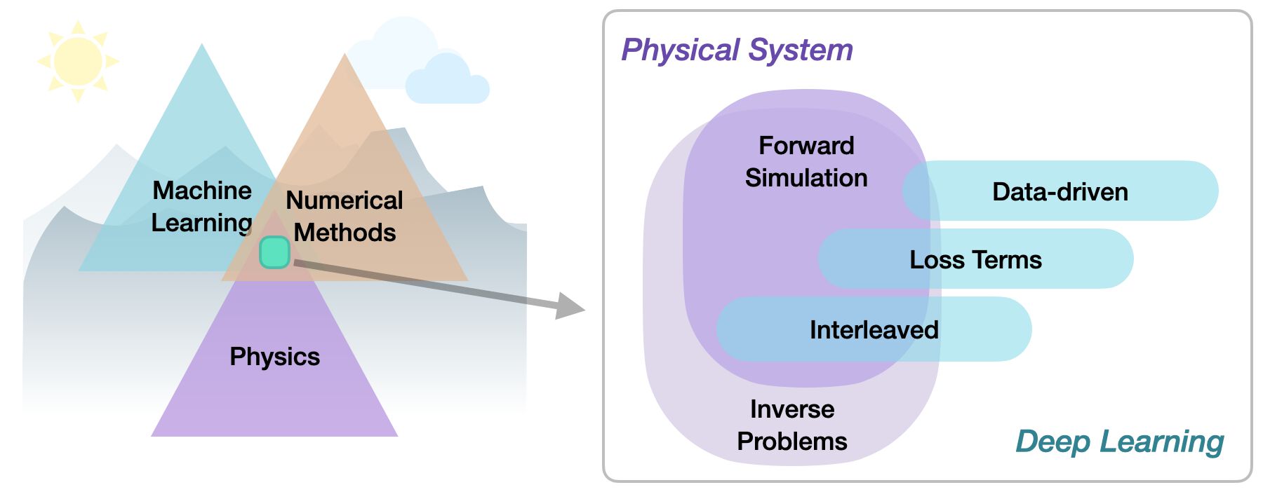
No matter whether we’re considering forward or inverse problem, the most crucial differentiation for the following topics lies in the nature of the integration between DL techniques and the domain knowledge, typically in the form of model equations via partial differential equations (PDEs). Taking a global perspective, the following three categories can be identified to categorize physics-based deep learning (PBDL) techniques:
Supervised: the data is produced by a physical system (real or simulated), but no further interaction exists. This is the classic machine learning approach.
Loss-terms: the physical dynamics (or parts thereof) are encoded in the loss function, typically in the form of differentiable operations. The learning process can repeatedly evaluate the loss, and usually receives gradients from a PDE-based formulation. These soft-constraints sometimes also go under the name “physics-informed” training.
Interleaved: the full physical simulation is interleaved and combined with an output from a deep neural network; this requires a fully differentiable simulator and represents the tightest coupling between the physical system and the learning process. Interleaved differentiable physics approaches are especially important for temporal evolutions, where they can yield an estimate of future behavior of the dynamics.
Thus, methods can be roughly categorized in terms of forward versus inverse solve, and how tightly the physical model is integrated into the optimization loop that trains the deep neural network. Here, especially the interleaved approaches that leverage differentiable physics allow for very tight integration of deep learning and numerical simulation methods.
More specifically
Physical simulations are a huge field, and we won’t cover all possible types of physical models and simulations in the following.
{note} Rather, the focus of this book lies on: - _Field-based simulations_ (no Lagrangian methods) - Combinations with _deep learning_ (plenty of other interesting ML techniques, but not here) - Experiments as _outlook_ (i.e., replace synthetic data with real-world observations)
It’s also worth noting that we’re starting to build the methods from some very fundamental building blocks. Here are some considerations for skipping ahead to the later chapters.
```{admonition} Hint: You can skip ahead if… :class: tip
you’re very familiar with numerical methods and PDE solvers, and want to get started with DL topics right away. The {doc}
supervisedchapter is a good starting point then.On the other hand, if you’re already deep into NNs&Co, and you’d like to skip ahead to the research related topics, we recommend starting in the {doc}
physicallosschapter, which lays the foundations for the next chapters.
A brief look at our notation in the
{doc}notation chapter won’t hurt in both cases, though!
```
Implementations
This text also represents an introduction to a wide range of deep learning and simulation APIs. We’ll use popular deep learning APIs such as pytorch https://pytorch.org and tensorflow https://www.tensorflow.org, and additionally give introductions into the differentiable simulation framework ΦFlow (phiflow) https://github.com/tum-pbs/PhiFlow. Some examples also use JAX https://github.com/google/jax. Thus after going through these examples, you should have a good overview of what’s available in current APIs, such that the best one can be selected for new tasks.
As we’re (in most jupyter notebook examples) dealing with stochastic optimizations, many of the following code examples will produce slightly different results each time they’re run. This is fairly common with NN training, but it’s important to keep in mind when executing the code. It also means that the numbers discussed in the text might not exactly match the numbers you’ll see after re-running the examples.