MIT Course 18.065/18.0651, Spring 2023
This is a repository for the course 18.065: Matrix Methods in Data Analysis, Signal Processing, and Machine Learning at MIT in Spring 2023. See also 18.065 from spring 2018 (MIT OpenCourseWare) for a previous version of this class.
Instructor: Prof. Steven G. Johnson.
Lectures: MWF1 in 2-190. Handwritten notes are posted, along with video recordings (MIT only).
Office hours (virtual): Thursdays at 4pm via Zoom.
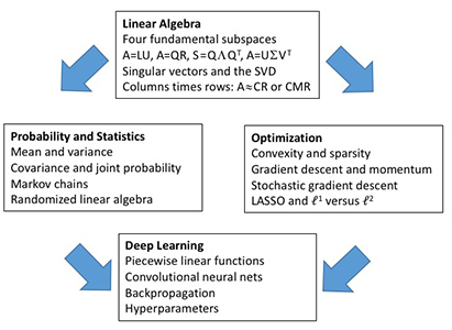
Textbook: Linear Algebra and Learning from Data by Gilbert Strang (2019). (Additional readings will be posted in lecture summaries below.)
Resources: Piazza discussion forum, pset partners.
Grading: 50% homework, 50% final project.
Homework: Biweekly, due Fridays (2/17, 3/3, 3/17, 4/7, 4/21, 5/5) on Canvas. You may consult with other students or any other resources you want, but must write up your solutions on your own.
Exams: None.
Final project: Due May 15 on Canvas. You can work in groups of 1–3 (sign up on Canvas). * 1-page proposal due Monday April 3 on Canvas (right after spring break), but you are encouraged to discuss it with Prof. Johnson earlier to get feedback. * Pick a problem involving “learning from data” (in the style of the course, but not exactly the same as what’s covered in lecture), and take it further: to numerical examples, to applications, to testing one or more solution algorithms. Must include computations (using any language). * Final report due May 15, as an 8–15 page academic paper in the style template of IEEE Transactions on Pattern Analysis and Machine Intelligence. * Like a good academic paper, you should thoroughly reference the published literature (citing both original articles and authoritative reviews/books where appropriate [rarely web pages]), tracing the historical development of the ideas and giving the reader pointers on where to go for more information and related work and later refinements, with references cited throughout the text (enough to make it clear what references go with what results). (Note: you may re-use diagrams from other sources, but all such usage must be explicitly credited; not doing so is plagiarism.) See some previous topic areas.
What followes is a brief summary of what was covered in each lecture, along with links and suggestions for further reading. It is not a good substitute for attending lecture, but may provide a useful study guide.
Lecture 1 (Feb 6)
- Syllabus (above) and introduction.
- Column space, basis, rank, rank-1 matrices, A=CR, and AB=∑(col)(row)
- See handwritten notes and lecture video linked above.
Further reading: Textbook 1.1–1.3. OCW lecture 1
Lecture 2 (Feb 8)
- Matrix multiplication by blocks and columns-times-rows. Complexity: standard algorithm for (m×p)⋅(p×n) is Θ(mnp): roughly proportional to mnp for large m,n,p, regardless of how we rearrange it into blocks. (There also exist theoretically better, but highly impractical, algorithms.)
- Briefly reviewed the “famous four” matrix factorizations: LU, diagonalization XΛX⁻¹ or QΛQᵀ, QR, and the SVD UΣVᵀ. QR and QΛQᵀ in the columns-times-rows picture, especially QΛQᵀ (diagonalization for real A=Aᵀ) as a sum of symmetric rank-1 projections.
- The four fundamental subspaces for an m×n matrix A of rank r, mapping “inputs” x∈ℝⁿ to “outputs” Ax∈ℝᵐ: the “input” subspaces C(Aᵀ) (row space, dimension r) and its orthogonal complement N(A) (nullspace, dimension n–r); and the “output” subspaces C(A) (column space, dimension r) and its orthogonal complement N(Aᵀ) (left nullspace, dimension m–r).
- pset 1, due Friday Feb 17
Further reading: Textbook 1.3–1.6. OCW lecture 2. If you haven’t seen matrix multiplication by blocks before, here is a nice video.
Optional Julia Tutorial: Wed Feb 8 @ 5pm via Zoom
- Virtually via Zoom. See the recording (MIT only).
A basic overview of the Julia programming environment for numerical computations that we will use in 18.06 for simple computational exploration. This (Zoom-based) tutorial will cover what Julia is and the basics of interaction, scalar/vector/matrix arithmetic, and plotting — we’ll be using it as just a “fancy calculator” and no “real programming” will be required.
- Tutorial materials (and links to other resources)
If possible, try to install Julia on your laptop beforehand using the instructions at the above link. Failing that, you can run Julia in the cloud (see instructions above).
Lecture 3 (Feb 10)
- Orthogonal bases and unitary matrices “Q”.
Choosing the right “coordinate system” (= “right basis” for linear transformations) is a key aspect of data science, in order to reveal and simplify information. The “nicest” bases are often orthonormal. (The opposite is a nearly linearly dependent “ill-conditioned” basis, which can greatly distort data.)
Orthonormal bases ⟺ QᵀQ=I, hence basis coefficients c=Qᵀx from dot products. QQᵀ is orthogonal projection onto C(Q). A square Q with orthonormal columns is known as a “orthogonal matrix” or (more generally) as a “unitary matrix”: it has Qᵀ=Q⁻¹ (both its rows and columns are orthonormal). Qx preserves length ‖x‖=‖Qx‖ and dot products (angles) x⋅y=(Qx)⋅(Qy). Less obviously: any square matrix that preserves length must be unitary.
Some important examples of unitary matrices: * 2×2 rotation matrices * the identity matrix I * any permutation matrix P which re-orders a vector, and is simply a re-ordering of the rows/cols of I * Hadamard matrices: unitary matrices Hₙ/√n where Hₙ has entries of ±1 only. For n=2ᵏ they are easy to construct recursively, and are known as Walsh–Hadamard transforms. * discrete Haar wavelets, which are unitary after a diagonal scaling and consist of entries ±1 and 0. They are a form of “time-frequency analysis” because they reveal information about both how oscillatory a vector is (“frequency domain”) and where the oscillations occur (“time domain”). * orthonormal eigenvectors can be found for any real-symmetric (“Hermitian”) matrix A=Aᵀ: A=QΛQᵀ * the SVD A=UΣVᵀ of any matrix A gives (arguably) the “best” orthonormal basis U for C(A) and the “best” orthonormal basis V for C(Aᵀ), which reveal a lot about A. * orthonormal eigenvectors can also be found for any unitary matrix! (The proof is similar to that for Hermitian matrices, but the eigenvalues |λ|=1 in this case.) Often, unitary matrices are used to describe symmetries of problems, and their eigenvectors can be thought of as a kind of “generalized Fourier transform”. (All of the familar Fourier transforms, including Fourier series, sine/cosine transforms, and discrete variants thereof, can be derived in this way. For example, the symmetry of a circle gives the Fourier series, and the symmetry of a sphere gives a “spherical-harmonic transform”.) For example, eigenvectors of a cyclic shift permutation give the discrete Fourier transform, which is famously computed using FFT algorithms.
Further reading: Textbook section 1.5 (orthogonality), 1.6 (eigenproblems), and 4.1 (Fourier); OCW lecture 3. The fact that preserving lengths implies unitarity is not obvious, but is proved in various textbooks; a concise summary is found here. The relationship between symmetries and Fourier-like transforms can be most generally studied through the framework of “group representation theory”; see e.g. textbooks on “group theory in physics” like Inui et al. (1996). Of course, there are whole books just on the discrete Fourier transform (DFT), just on wavelet transforms, etcetera, and you can find lots of material online at many levels of sophistication.